


Ford-Fulkerson Algorithm
A Step-by-Step Guide to Max Flow

Hello! This post is a follow-up of 1,000 Subscribers, 1 Coding Challenge!, where we announced a coding challenge. Today, we will explore one possible solution: the Ford-Fulkerson algorithm. The solution will be given at the end.

Understanding the Max Flow Problem
The maximum flow problem involves finding the highest possible flow that can travel from a source to a sink in a flow network without exceeding edge capacities.
Key terminology:
Flow: The amount of “stuff“ (e.g., water, data, cars) passing through an edge without exceeding the edge’s capacity.
Capacity: The maximum amount of flow an edge can handle.
Vertex: A node in the network where the flow can enter or exit.
Edge: A directed connection between two vertices that carries flow and has a capacity limit.
Source: The starting point of the flow, where all the "stuff" originates.
Sink: The endpoint where all the "stuff" is collected.
Some real-world applications:
Water pipeline system: A network of pipes where water flows from a reservoir to homes with pipes having different capacities. What’s the maximum water flow that can be transported?
Data networks: Internet packets traveling through routers, where each connection has a bandwidth limit. What’s the maximum throughput between two routers?
Traffic flow: Routes connecting cities, where cars move from an entry point to an exit, and each route has a capacity limit. What’s the maximum number of cars that can travel between two cities?
Augmenting Path
Before diving into the algorithm, we first need to define the concept of augmenting path:
A path from the source to the sink is a sequence of connected vertices that begins at the source and ends at the sink.
An augmenting path is a path from the source to the sink in which every edge has available capacity for additional flow.
For example:

A → B → Dis both a valid path and an augmenting path because all edges along the path have remaining capacity.A → C → Dis a valid path but not an augmenting batch becauseC → Dhas no remaining capacity, meaning no additional flow can pass through this path.
Ford-Fulkerson Algorithm
Consider the following graph where we need to find the maximum flow from A to F:

Intuition Behind the Algorithm
One possible intuition for solving this problem could be:
Find an augmenting path from
AtoF(i.e., a valid path where all the edges have remaining capacity).Calculate the bottleneck capacity—the maximum flow that this path can carry, limited by the edge with the smallest available capacity.
Update the capacity of the edges along this path by subtracting the bottleneck flow.
Repeat steps 1-3 until no more augmenting paths exist.
Let’s follow this intuition and apply it step by step.
Finding Augmenting Paths
Note that the Ford-Fulkerson algorithm doesn’t impose a specific way to find augmenting paths. For this example, we use Depth-First Search (DFS).
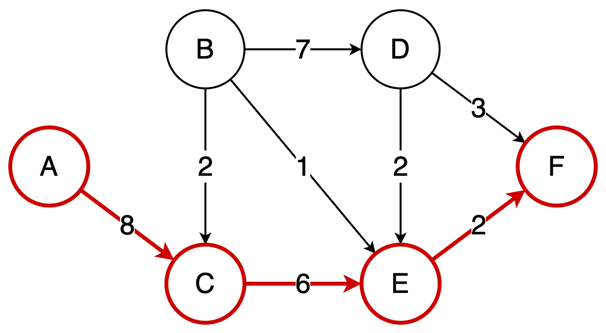
Suppose the first augmenting path found is A → B → E → F:

The bottleneck for this path is 2 as any additional flow would exceed A → B capacity.
We push a flow of 2 through this path. Then, to reflect on the flow that has been sent, we update the remaining capacity of all edges in this path by removing 2:

Capacity updates:
A → B: The capacity went from 2 to 0 (-2), so we removed the edge. We could also keep a capacity of 0; it doesn’t really matter.B → E: The capacity went from 3 to 1 (-2).E → F: The capacity went from 4 to 2 (-2).
Now, let’s find another augmenting path using the same technique, DFS. Suppose the next path found is A → C → E → F:
The bottleneck for this path is 2 (bounded by E → F). So again, we update the remaining capacity of all the edges in this path:

Capacity updates:
A → C: The capacity went from 8 to 6 (-2).C → E: The capacity went from 6 to 4 (-2).E → F: The capacity went from 2 to 0 (-2), so we removed the edge.
A Correct Solution?
At this stage, there is no more augmenting path left from A to F. Let’s summarize:
We found a first augmenting path
A → B → E → Fwith a max flow of 2.We found a second augmenting path
A → C → E → Fwith a max flow of 2.
Therefore, if our intuition was correct, the maximum flow between A and F should be 4. However, this isn’t the right solution. Instead, we should have considered these two augmenting paths:
A → B → D → F: 2A → C → E → F: 4
If we had taken these two augmenting paths, we would have found the correct solution: 6.
What Went Wrong?
Should we refine our way of selecting augmenting paths? Not with Ford-Fulkerson. As we said, augmented paths in Ford-Fulkerson can be selected arbitrarily, so let’s keep using DFS.
Instead, we’re missing a crucial step: whenever we select an augmented path and send flow through an edge, a backward edge with the same flow value must be created.
The purpose of this step is to allow flow redistribution, meaning if an unlucky selection of augmenting paths leads to a suboptimal result, the algorithm can undo and redistribute the flow when needed. Let’s see how that works.
Incorporating Backward Edges
We restart the algorithm to find the maximum flow from A to F, this time properly incorporating backward edges.
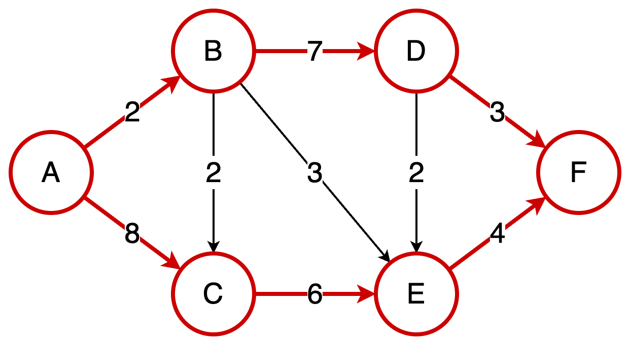
The first augmented path found is still A → B → D → F:
Now, instead of just adapting the capacity, we will create a backward edge based on the flow sent. In this case, the flow sent is 2 so we will create three backward edges with a capacity of 2:
Capacity updates:
A → B: The capacity went from 2 to 0 (-2), so we removed the edge.B → E: The capacity went from 3 to 1 (-2).E → F: The capacity went from 4 to 2 (-2).
Meanwhile, we added three backward edges with a capacity based on the flow sent (2):
B → A: 2E → B: 2F → E: 2
Why we’re doing this may not be clear yet, but let’s keep going—you will soon see why it makes sense.
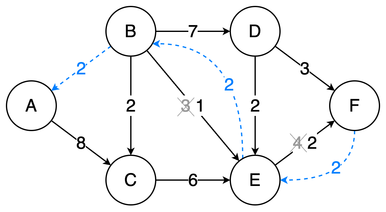
Now, let’s consider the second path, A → C → E → F:
The max flow for this path is 2. We follow the same steps by updating the capacity for all the edge in the path (-2) and all the backward edges (+2).
We update all the capacity and create 2 new backward edges:
C → A: 2E → C: 2
The F → E backward edge was already present from the first augmented path, so we increment its capacity: 2 + 2 = 4.
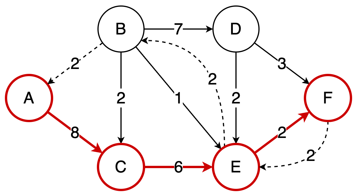
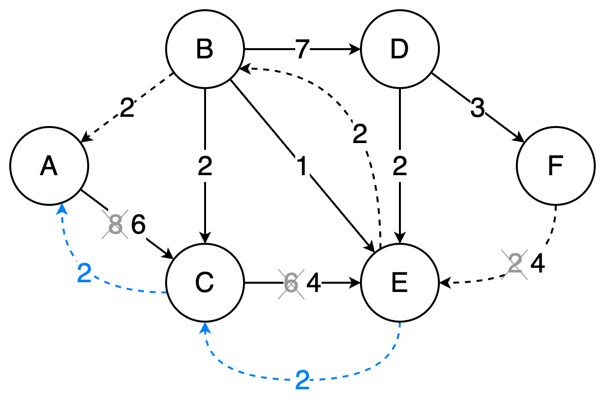
At this stage, we are at the same point as before, where we have found two augmenting paths with a flow of 2. However, there’s now a major difference: thanks to backward edges, there is one more remaining augmenting path: A → C → E → B → D → F. Note that this new path uses a backward edge that we created: E → B. Let’s consider this path:

The path’s bottleneck is 2 (bounded by E → B). Let’s adapt the capacities:
-2 for all the edges in the path (including
E → F).+2 for all the backward edges.

Note that as we decreased by 2 the capacity of E → B, it reached a capacity of 0, so we removed the edge.
Is there a remaining edge? No, that’s the termination condition of Ford-Fulkerson. Here are all the augmenting paths that we found and their corresponding flows:
A → B → E → F: 2A → C → E → F: 2A → C → E → B → D → F: 2
If we sum all the flows, we get 6, which is the correct maximum flow.
This is how the Ford-Fulkerson algorithm guarantees that, even with arbitrary augmenting path selection, it will always find the correct maximum flow thanks to backward edges allowing flow redistribution.
Code

Pseudo-code:
def ford_fulkerson(graph, source, sink):
    res = 0
    while True:
        path = get_next_augmenting_path(graph, source, sink)
        if path is None:
            break

        bottleneck = get_bottleneck(path)
        for edge in path.get_edges():
            edge.capacity -= bottleneck

            backward_edge = get_backward_edge(graph, edge)
            backward_edge.capacity += bottleneck

        res += bottleneck

    return res
You can also look at my Go solution.
Complexity
The time complexity of Ford-Fulkerson algorithm is O(EU), where:
Eis the number of edges in the graph.Uis the maximum possible flow (i.e., the solution).
It’s quite interesting to note that the algorithm’s complexity depends on the final solution itself. This is something fairly unusual because, ideally, we don’t want to solve the problem first just to determine its time complexity.
We can, however, approximate U, as it depends on the edge capacities. If we increase the edge capacities, then in most cases, the maximum flow U will also increase. Yet, this isn’t the only factor and we should also consider:
Bottlenecks: If a single edge has low capacity, it limits
Uno matter how large other edges are.Graph structure: Even if edges have large capacities, if there are few paths from source to sink,
Umay not be very large.Parallel paths: If there are many disjoint paths from the source to the sink,
Uwill be higher even if individual edges have small capacities.
Yet, one important question: What if we need an algorithm whose complexity doesn’t depend on U since U isn’t straightforward to estimate?
Amazingly, the solution is to simply change how we determine augmenting paths. In our example, we used DFS, which led to an O(EU) complexity. However, if we switch Breadth-First Search (BFS) instead, the time complexity becomes O(VE²), where:
Vis the number of vertices (nodes) in the graph.Eis the number of edges in the graph.
Said differently, with BFS, the time complexity depends only on the graph structure (vertices and edges). This removes the difficulty of predicting an accurate value of U.
This specialization of Ford-Fulkerson using BFS is known as the Edmonds-Karp algorithm.
Summary
Ford-Fulkerson repeatedly finds augmenting paths and pushes flow through them.
Backward edges allow redistribution of flow, which corrects any suboptimal choices made by selecting arbitrary augmenting paths.
The algorithm terminates when no more augmenting paths exist.
Using DFS, the time complexity is
O(EU), which depends on the final solution, but switching to BFS (Edmonds-Karp variation) results in a time complexity ofO(VE²), making it dependent only on the graph structure.
❤️ If you made it this far and enjoyed the post, please consider giving it a like.

📚 Resources
More From the Coding Category
Sources
Maximum flow problem - Ford Fulkerson algorithm // The graph example I used in this post is taken from this video. If you struggle with my explanation, this video may help you.
Explore Further
Dinic’s Algorithm - YouTube // An explanation of Dinic’s network flow algorithm, another way to solve max flow problems.
🎉 Solution
The correct solution to the 1,000 Subscribers, 1 Coding Challenge! was 56. Congratulations to everyone who solved it! The winners (Simon, María, Alexandr, Brian, Vadim), chosen randomly from all correct submissions, will be notified by email.
Thanks to all who participated! I hope you enjoyed the challenge. Let me know if you'd like to see more of these in the future!